azure-vpn

记录常见的 激活函数 以及 损失函数

激活函数

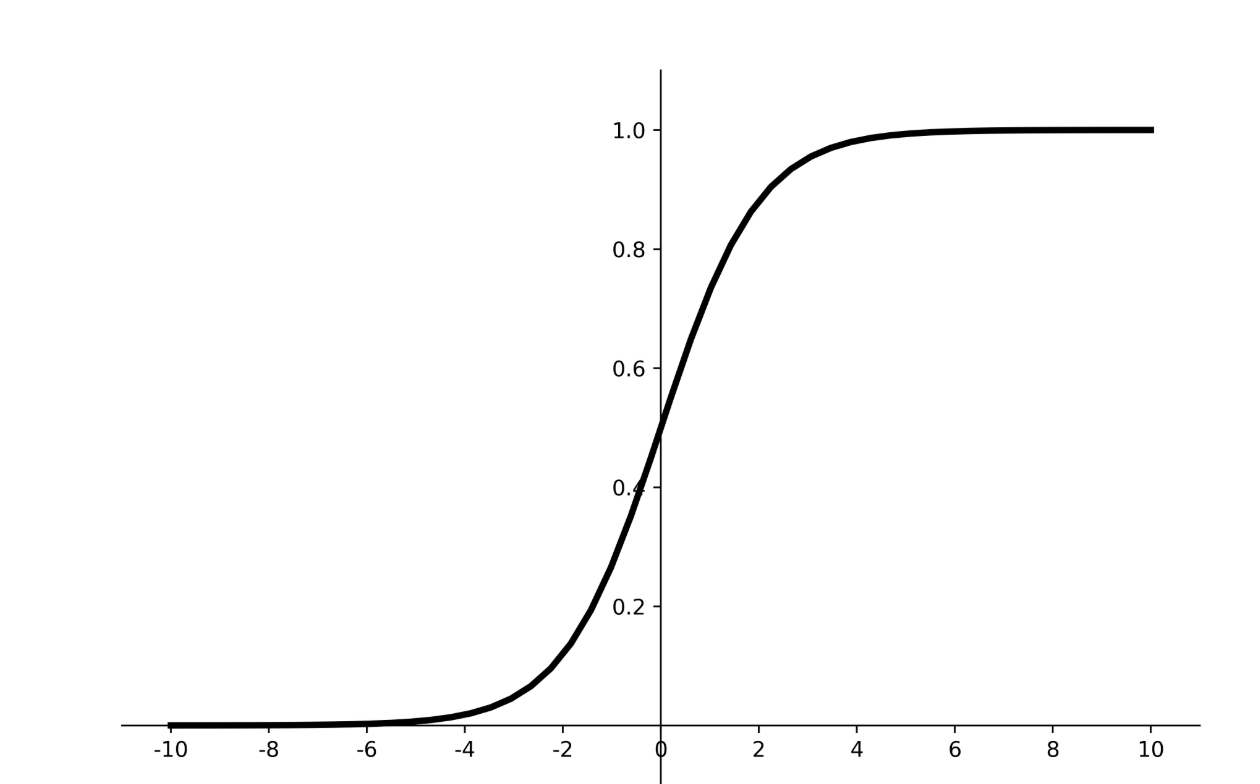
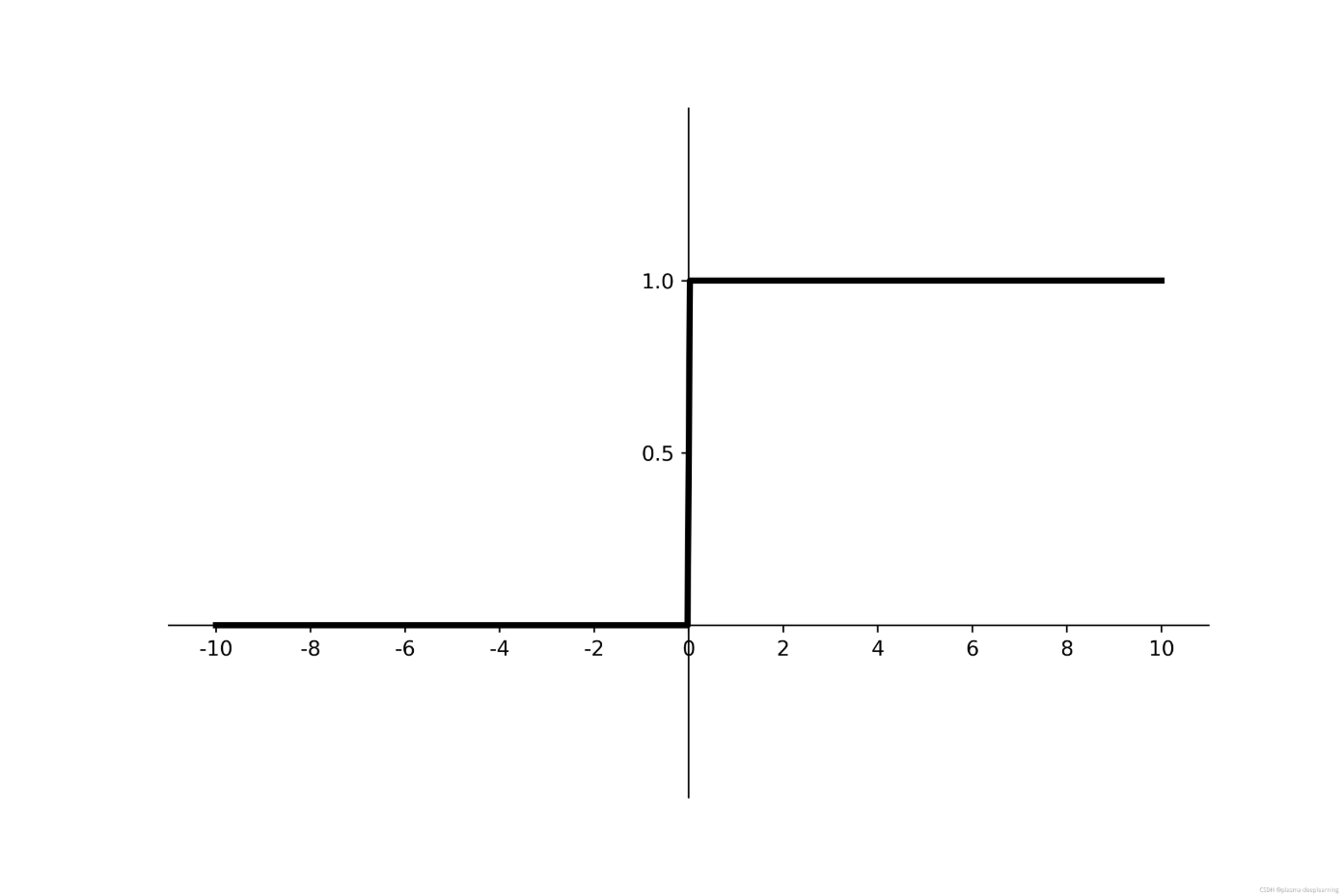
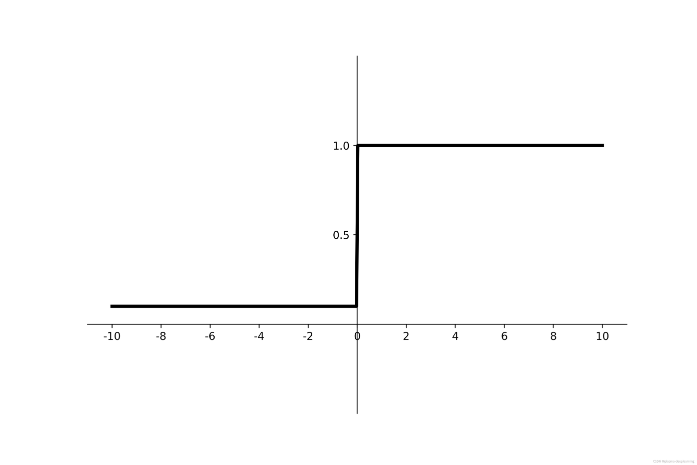
Sigmoid

f(x) = 1/(1+e^(-x))

$$ f(x)=\frac{1}{1+e^{-x}} $$

f(0) = 0.5 ,f(x) 取值范围在 (0,1) 之间

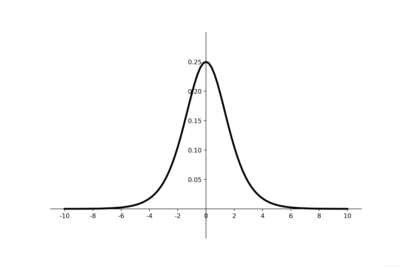
导数为:

f'(x) = f(x) - (1-f(x))

$$ f’(x)= f(x) - (1-f(x)) $$

图像如下:

优点： 1、 输出映射在(0,1)之间，单调连续，输出范围有限，优化稳定，可用作输出层； 2、求导容易。 缺点： 1、易造成梯度消失； 2、输出非0均值，收敛慢； 3、幂运算复杂，训练时间长。

sigmoid 只适用于二分类问题，不适用于多分类问题

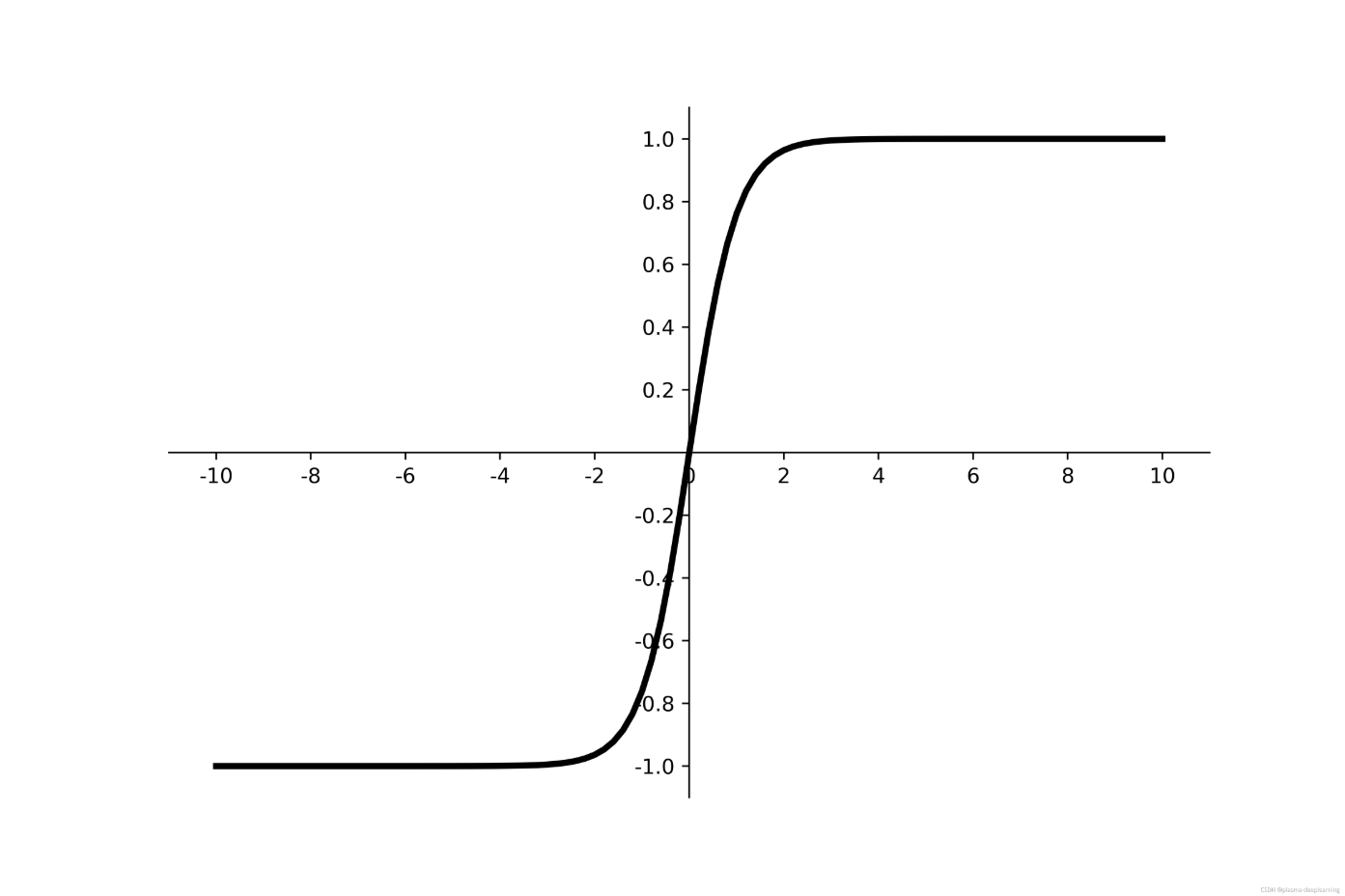
tanh

f(x) = (e^x - e^(-x)) / (e^x +e^(-x))

$$ f(x)=\frac{(e^x-e{-x})} {e^x +e^{-x}} $$

取值范围为：(0,1)

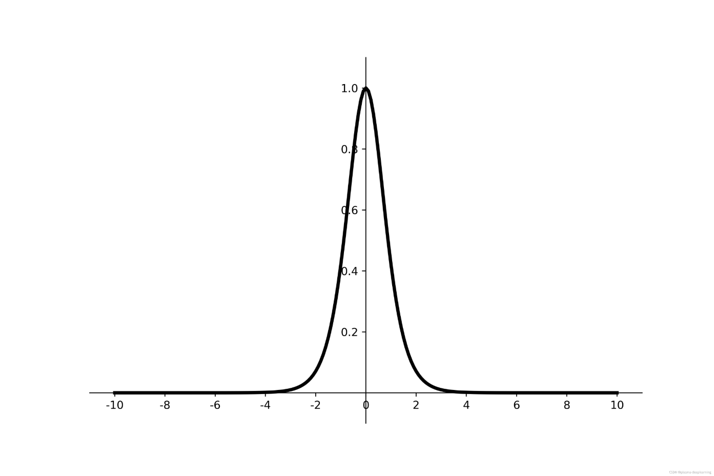
导数为:

f'(x) = 1 - f(x)^2

$$ f’(x) = 1 -f(x)^2 $$

优点：

1. 比sigmoid函数收敛速度更快。
2. 相比sigmoid函数，其输出以0为中心。

缺点：

1. 易造成梯度消失；
2. 幂运算复杂，训练时间长。

Softsign

f(x) = x/(1 + |x|)

取值范围： (-1,1)

f'(x) = 1/(1+x)^2

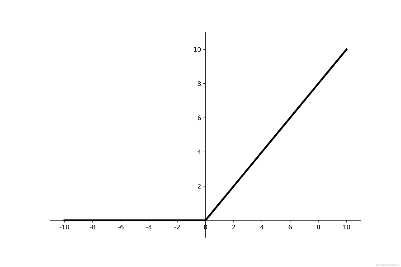
ReLU

f(x) = max(0,x)

$$ f(x) = \begin{cases} 0, & x < 0 \ x, & x \ge 0 \end{cases} $$

f(x)取值范围为 (0，+00)

导数为:

f'(x) = max(0,1)

$$ f’(x)=max(0,1) $$

优点：

解决了梯度消失问题(在正区间)； 只需判断输入是否大于0，计算速度快； 收敛速度远快于sigmoid和tanh，因为sigmoid和tanh涉及很多expensive的操作； 提供了神经网络的稀疏表达能力。

缺点：

输出非0均值，收敛慢； 神经元死亡：某些神经元可能永远不会被激活，导致相应的参数永远不能被更新。

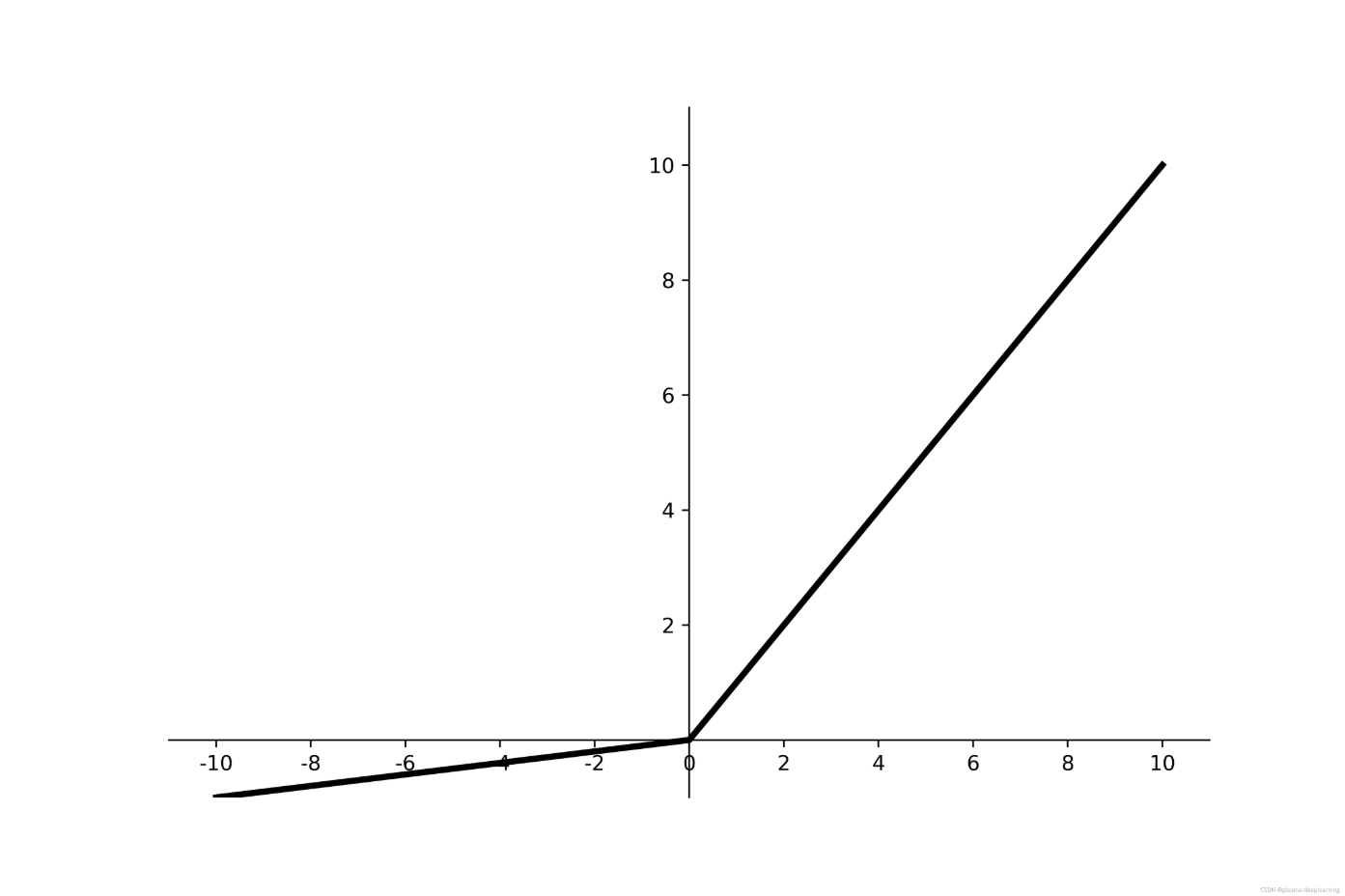
Leaky-ReLU

if x >= 0： 
	f(x) =  x ;
if x < 0:
	f(x) = ax ; 

取值范围 (-00,+00);P-ReLU则认为 a 也应当作为一个参数来学习，一般建议初始化为0.25。

导数为:

if x >= 0;
	f'(x) = 1 ;
if x <= 0;
	f'(x) = a;

理论上来讲，Leaky ReLU有ReLU的所有优点，外加不会有神经元死亡的问题，但是在实际操作当中，并没有完全证明Leaky ReLU总是好于ReLU。

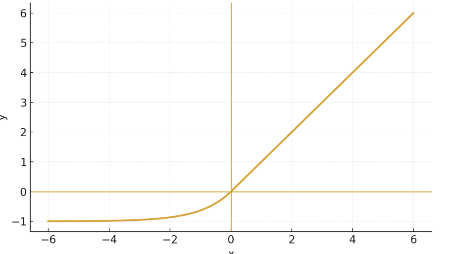
GeLU

原始公式 $$ \begin{equation} \mathrm{GELU}(x) = x \cdot \Phi(x) \

\text{其中} \space \Phi(x) = \frac{1}{2}\left[1 + \operatorname{erf}!\left(\frac{x}{\sqrt{2}}\right)\right]

\end{equation} $$

合并

$$ \begin{equation} \mathrm{GELU}(x)

x \cdot \frac{1}{2}\left[1 + \operatorname{erf}!\left(\frac{x}{\sqrt{2}}\right)\right] \end{equation} $$

但是实际的训练时使用的是近似的公式 $$ \begin{equation} \mathrm{GELU}(x)

\frac{x}{2} \left( 1 + \tanh \left( \sqrt{\frac{2}{\pi}} \left( x + 0.044715 x^{3} \right) \right) \right) \end{equation} $$

便是这样的情况

$$ \begin{align} \mathrm{GELU}(x) &= x \cdot \Phi(x) \ &= x \cdot \frac{1}{2}\left[1 + \operatorname{erf}!\left(\frac{x}{\sqrt{2}}\right)\right] \ &\approx \frac{x}{2}\left(1 + \tanh\left(\sqrt{\frac{2}{\pi}}\left(x + 0.044715 x^{3}\right)\right)\right) \end{align} $$

SwiGLU

$$

$$

ELU

if x >= 0:
	f(x) = x;
if x < 0:
	f(x) = a(e^x - 1);

$$ \text{ELU}(x) = \begin{cases} x, & x \ge 0 \ \alpha \left(e^x - 1\right), & x < 0 \end{cases} $$

Softmax

公式为：

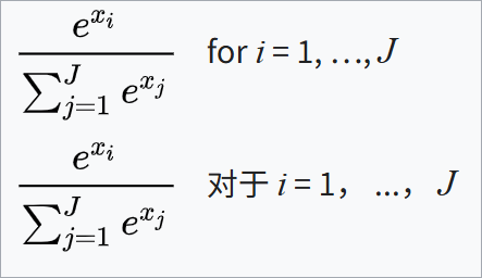
• 矩阵形式

$$ \text{Softmax}(\mathbf{z}) = \frac{e^{{\mathbf{z}}}{\sum_{j=1}}{n} e^{z_j}} $$

损失函数

均方误差损失函数 MSE

MSE, Mean Squared Error

$$ L(Y|f(x))=\frac{1}{n}\sum_{i=1}{N} (Y_i-f(x_i))^2 $$

• pytorch 使用

import torch
y = torch

交叉熵损失 CrossEntropyLoss

总的函数 $$ L = -\sum_{i=1}^{n} y_i \log(\hat{y}_i) $$

• 单样本交叉熵

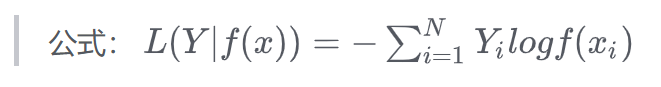
$$ L = -\sum_{i=1}^{n} y_i \log(\hat{y}_i) $$

• 多样本平均损失

$$ L = -\frac{1}{m}\sum_{k=1}^{{m}\sum_{i=1}}{n} y_{k,i}\log(\hat{y}_{k,i}) $$

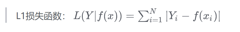
L1 损失

L2 损失

KL散度

KL 散度（Kullback–Leibler Divergence）

应用场景：VAE（变分自编码器）中衡量分布差异。

解释：越小代表两个分布越接近。 $$ D_{KL}(P|Q) = \sum_i P(i) \log \frac{P(i)}{Q(i)} $$